1 Introduction
This century has so far been one of severe disruption for the recorded music industry. In 1999, the arrival of online file sharing service Napster heralded the beginning of the end for the recording industry’s established business model. After peaking at $21.5bn in 1999, US recorded music revenues collapsed to just $6.9bn in 2015.[1] In the last three years, however, revenues have started to rise again, driven by the explosive growth of music streaming services such as Apple Music and Spotify.
The surge in popularity of music streaming offers leading service providers a wealth data on consumer preferences and listening habits. By harnessing this newly available data, providers can improve user experience and maintain a competitive edge over rival platforms. An important feature for streaming services is customised music recommendations, and the effectiveness of these recommendations depends heavily on the ability to accurately predict a song’s popularity.
This paper will aim to develop a model for predicting a song’s popularity using data from Spotify. We consider eight potential predictor variables for a song’s popularity, and after performing uni-variate and bi-variate analyses, seek fit an optimal linear model to the data. After selecting the model, we assess the validity of the model’s assumptions, and then use the model to predict a song’s popularity given new data.
2 Data Description
To obtain the data used for analysis a function was used that accesses Spotify’s database and extracts the songs for a list of artists given to it. The decade variable is added manually to each of the artists. These artists where chosen to be a representation of their respective decade; namely Elvis Presley, The Beatles, David Bowie, Micheal Jackson, Blur and Beyonce, representing the 50s, 60s, 70, 80s, 90, and 00s respectively.
The raw data contains 2081 observations of 21 variables. This initial data scrape is reduced in scope to the following variables:
| Types | Variables |
|---|---|
| Identifiers | Track Name, Artist |
| Metrics | Popularity, Danceability, Energy, Loudness, Duration |
| Catagories | Key, Mode, Time Signature, Decade |
3 Cleaning
3.1 Loading and Type Assignment
Prior to analysis the data is loaded into the R studio environment and inspected to ensure that subsequent operations are applied to a consistent and uniform dataset. To achieve this, the variables that are out of scope in this analysis are removed. Each of the remaining categorical variables are inspected to ensure their levels are ordered correctly within each factor. Re-leveling was only necessary for the decade variable due to its chronological nature giving it an ordinal structure. The remaining factors’ levels were left in alphabetical or numerical order as they are non-ordinal or this default ordering preserves their inherent order. Each of the newly created factor levels were then tabulated. Initially a time signature of zero was considered to be erroneous, but when reviewing the reference material it is not a known fixed quantity, as is with most sheet music. The value is estimated for the track by an algorithm, thus multiple rests or lack of percussion may lead to the estimated time signature falling bellow one and being rounded to zero.[2] Due to this no remediation was used on the samples contained in this level.
3.2 Missing Values
Leveled factors and numerical variables are then subjected to missing value analysis to ensure samples are described completely. To do this, frequency counts for empty, non-applicable and null variable values across the dataset were extracted to produce a bar chart with each variable’s respective missing value content shown as a percentage, . This analysis revealed that none of the variables that will be used in the analysis are missing any values.
As missing values in numerical data can often be encoded as zeros, these variables where tested for zero content. This revealed that the highest zero value content, 3.5%, is observed in the Popularity variable and 0.25% where found in the case of danceability. These low levels of zero content are likely appropriate for the given variables and are left unchanged.
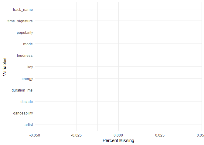 | 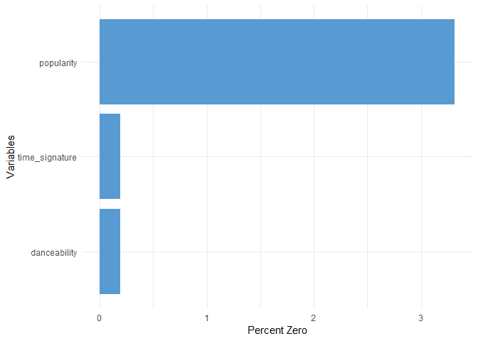 |
Bar charts showing the frequency of missing values (left) and zero values (right) as a percentage of overall observations.
The cleaned data has 2081 observations of 11 variables. However, two of the remaining variables are retained for interpretation and labeling only, namely Artist and Track Name, leaving 9 possible predictors.
4 Description of Variables
4.1 Continuous Variables
Popularity appears to be bi-modal, with modes at 0 and 20. The mode present at zero might be due to a minimum threshold required before being rated on the interval from [0-100]. The majority of examples are present after the second mode giving the overall distribution a slight skew towards the right, (left).
Loudness has a single mode at around -5 with most examples lying to the left of the mode. This skews the distribution to the left. The distribution has a low kurtosis, evidenced by the lack of a sharp mode, (right).
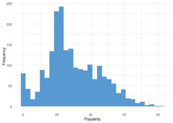 | 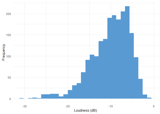 |
Histograms of the popularity (left) and loudness (right) variables imported from Spotify.
Energy has an extremely low kurtosis, to the point that no easily identifiable mode. The examples are roughly uniformly distributed over the interval [0.3, 0.9] with a steep drop off in frequency either side of this interval, (left).
Danceability displays a distribution that is approximately normal. There is a single mode at 0.6 and the kurtosis of the distribution appears to be normal, (right).
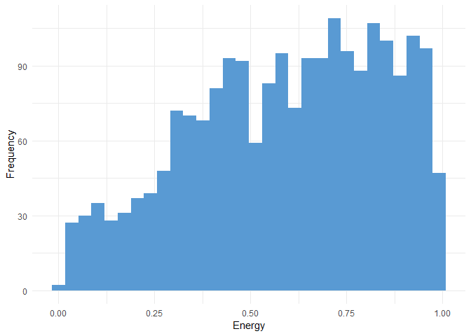 | 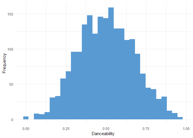 |
Histograms of the Energy (left) and Danceability (right) variables imported from Spotify.
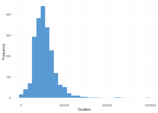
The figure above is a histogram of the Duration variable, which is the duration of songs in the Spotify dataset, measured in milliseconds. The distribution is unimodal with high kurtosis. There is a slight positive skew, with apparent outliers at the higher end of the distribution.
4.2 Catagorical Variables
(left) indicates that Key has a strong mode in category C with other frequently sampled categories A, D and G. The Categories D#, F#, G# are the least likely key for a song to be in. Mode shows a strong preference for songs to be written in major key as apposed to a minor.
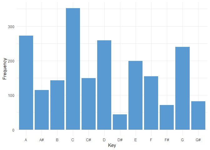 | 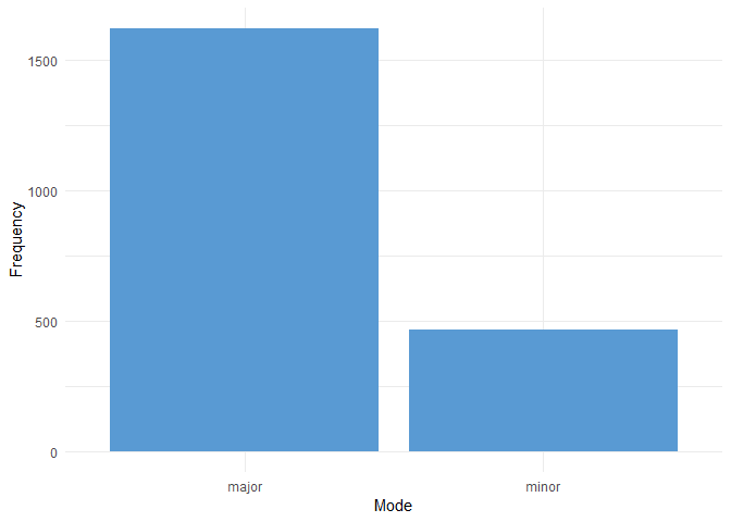 |
Bar charts of the Key (left) and Mode (right) variables imported from the Spotify set.
(left) shows the number of tracks grouped by their respective time signatures. The most common time signature observed is 4 with about 1800 tracks The second most common time signature is 3 with around 250 tracks. Very few tracks have time signatures of 0, 1 and 5. (right) shows the number of tracks with respect to each decade analysed. The most common decade that songs originated from is the 50s, followed by the 70s, with about 600 and 550 songs respectively. The 60s, 80s, 90s, and 00s all have approximately 150 to 250 songs each.
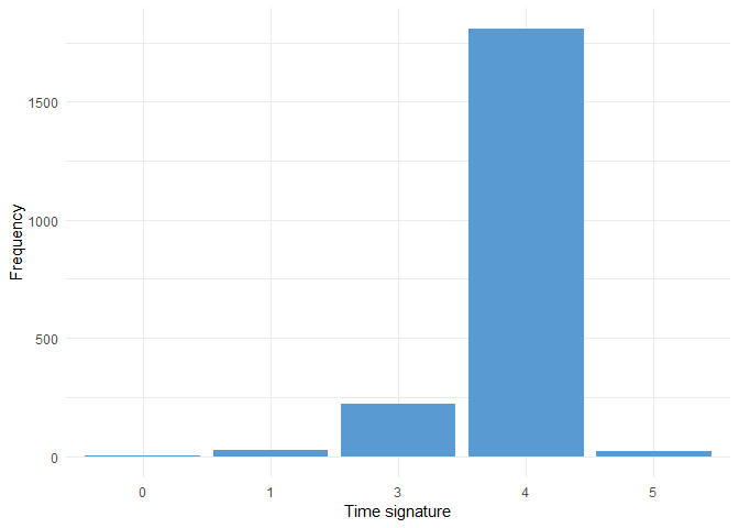 | 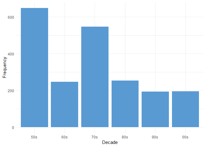 |
Barcharts of the Time Signature (left) and Decade (right) variables imported from the Spotify set.
5 Bivariate Analysis
Bi-variate analysis is the simultaneous analysis of two variables to explore the relationship between them. This section contains bi-variate analyses of the Popularity variable against eight potential predictor variables from the spotify dataset.
5.1 Continuous Variables
(left) shows a scatter plot of the Duration variable against Popularity. There appears to be very little association between the two variables, with no discernible direction, with data points appearing to be scattered randomly about the mean of Popularity. Their is no detectable non-linearity in the distribution of the data either. Four potential outliers are seen to appear down field, having high levels of Duration.
(right) appears to show no evidence of an association between the two variables, with the data points randomly scattered about the mean of Popularity. There is no indication of a nonlinear trend, or any outliers.
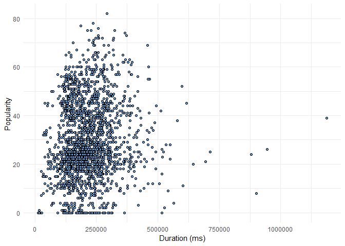 | 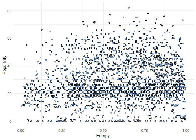 |
Scatter plots of the Duration (left) and Energy (right) variables against Popularity.
In (left) there appears to be a weak positive association between Popularity and Danceability, though there appears to be a strong concentration of samples around a popularity of 20 across a wide range of Danceability. There is no evidence of a nonlinear trend in the data, or any apparent outliers.
A weak positive association is also evident in (right) between Popularity and Loudness, with some indication of curvature in the relationship. Again a dense section of samples are seen around popularity’s mean that constitutes over a the range of values loudness has. Possible outliers may be present with lower levels of Loudness and higher Popularity scores. The variance of the Popularity score appears to be increasing for higher levels of Loudness.
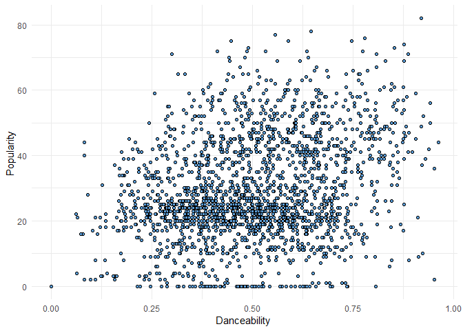 | 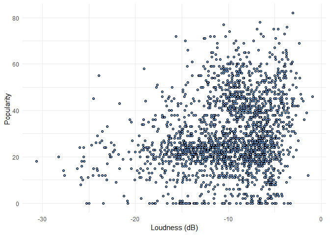 |
Scatter plots of the Danceability (left) and Loudness (right) variables against Popularity.
5.2 Categorical Variables
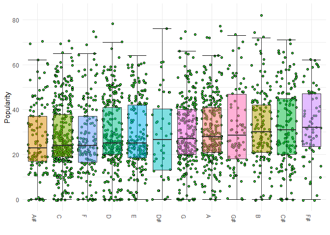 | 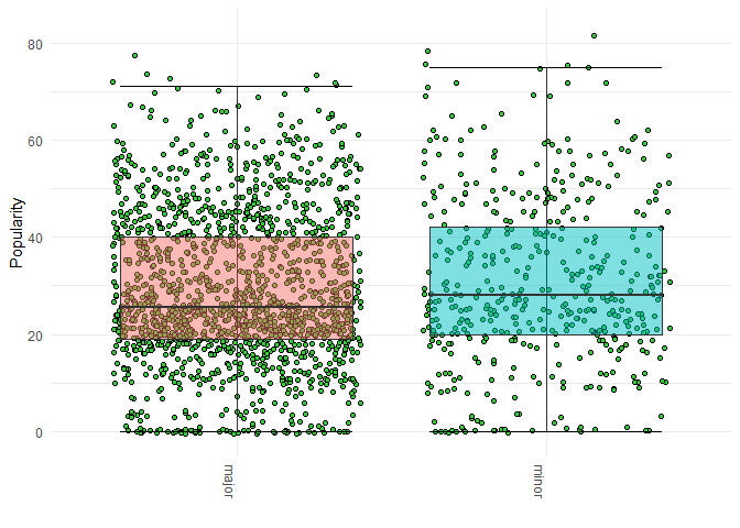 |
Box plots of sample Key (left) and Mode (right) variables against Popularity.
Across the series of keys there is very little variation in group mean and variance. Some groups are are slightly smaller in range than others, but the distributions appear uniform. The only aspect in which they differ greatly is the density of examples present in the different categories; the sharp keys all being particularly sparse, .
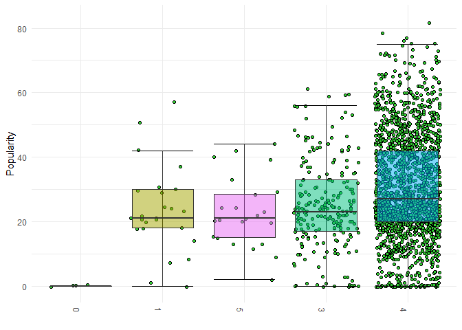 | 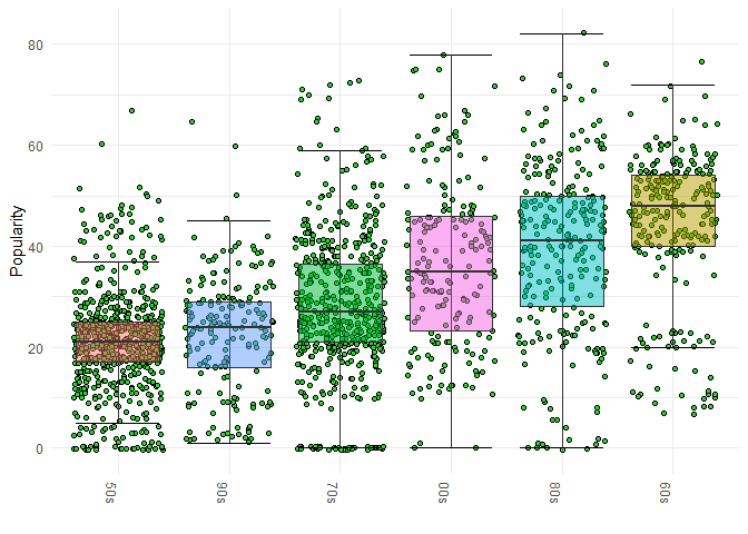 |
Box plots of sample Time Signatue (left) and Decade (right) variables against Popularity.
There is not much difference in the popularity between tracks with time signatures 1, 3 and 5. Tracks with a time signature of 4 appear slightly more popular than those with other time signatures. Tracks with a time signature of 0 have about 0 popularity. This may occur when a track has no sound or length. The largest difference between the time signatures is in the number of samples with that respective time signature, (left).
Across the decades, the 50s and the 70s have a particularly dense amount of observations clustered around their respective medians, while the 00s and the 80s data have more of a spread, with the 60s in between the two. The 60s have the highest median popularity level, while the 00s, 80s, and 70s to a lesser degree have the most popular individual songs, (right).
5.3. Bivariate Analysis Between Predictors
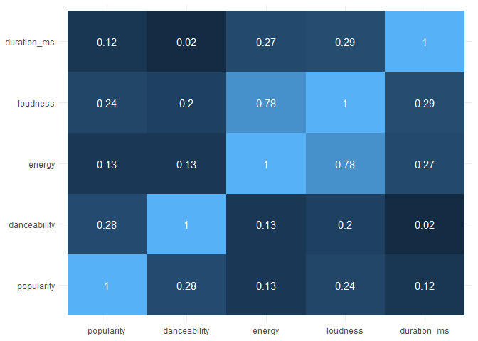
The correlation matrix above indicates a fairly strong correlation between the Energy and Loudness variables. No other variables look to have significant associations with one another.
Anova was used to inform the scope used in the subsequent model fitting processes. A specific scope was created with the terms identified as significant in the table. This was done to limit the available terms during modeling to those that already have a significant relationship between them and the predictor, reducing potential model complexity and computation. Additionally this excludes a large number of interaction terms that may otherwise be included in the model.
6 Model Fitting
To fit the linear model, forward, backward and step-wise algorithms for model selection were all used, with both the Akaike Information Criterion (AIC) and Bayesian Information Criterion (BIC) as heuristics. Each of the model selection algorithms iteratively adds and/or removes terms using appropriate measures of significance, until the optimal model has been identified. The model with all terms available for inclusion is called the full model. The model with the least possible terms is the null model.
The forward algorithm begins with the null model. At each iteration, the P-value is calculated for each term that is not currently included in the model. If the smallest P-value is less than a threshold (in our case 0.05), the term with that P-value is added to the model. The backward algorithm begins with the full model, and at each iteration, calculates the P-values for all terms in the model. If the highest P-value exceeds the chosen threshold, that term is removed from the model. This is repeated until all included terms are significant. The stepwise algorithm begins with the null model. At each iteration, one step of forward selection is performed, using a liberal P-value such as 0.20, and one step of backward elimination is performed using a lower P-value such as 0.05. This is repeated until no further changes occur in the model.
Three different full models were considered. The first full model included all predictors but no interaction terms. The second used only those terms, either individual predictors or interactions between them, that were identified as significant in the previous section. The third included all predictor terms and all interaction terms. The criteria scores and k-fold mean square error for models obtained using each algorithm and heuristic.
Using the first full model, where no interaction terms were included, led to the selection of the same best model irrespective of algorithm or heuristic. The AIC for this model was the highest overall. The BIC was somewhat lower, though not the lowest overall. The k-fold MSE scores were the highest. Given these results, this model was a poor candidate for final selection.
For the remaining two models, we found that the best models obtained from using the BIC heuristic contained substantially fewer terms than the those obtained under AIC. Despite being much smaller models, those obtained under the BIC heuristic were not penalised with higher significantly higher AIC or MSE scores. Therefore, it was determined that the final model would be selected from among those obtained using the BIC heuristic. Of these, the forward algorithm produced models with higher MSE than those of backward and step-wise. For the two remaining full models, backward and step-wise algorithms arrived at the same best model in each case. Of these two models, there was very little difference in MSE, so it was determined that the simplest model would be chosen as the final model.
7 Final Model
The results from the selection process indicate that the model obtained using the ‘only significant terms’ full model, then applying the backward (or step-wise) algorithm with the BIC heuristic, was the optimal choice. The formula for this model is:
popularity ~ decade + danceability + loudness + energy + duration_ms + , energy:duration_ms + decade:loudness
The interaction terms included in this model were judged to be meaningful and therefore reasonable to include in the model. Longer songs may be expected to exhibit a higher level of energy compared to shorter songs. Likewise, it is feasible that loudness of songs has changed in different decades, as decade is a proxy for Artist.
The coefficients for this model are presented in Table 5. The coefficients are the predicted change in popularity for an increase of 1 in the predictor term.
8 Assumption Checking
The assumptions of the final linear model are:
- Linearity. There exists a linear relationship between the target and predictor variables in the model.
- Homoscedasticity. The variance of the error terms is constant.
- Normality. The error terms are normally distributed with a mean of zero.
- Independence. Error terms are independent of one another.
These assumptions are checked using the plots below.
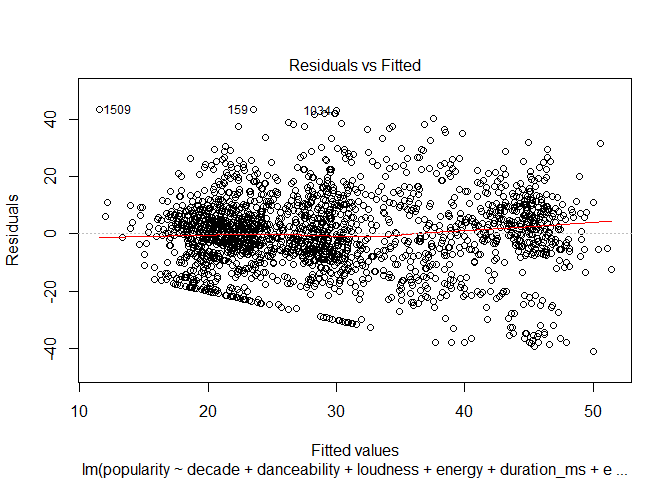 | 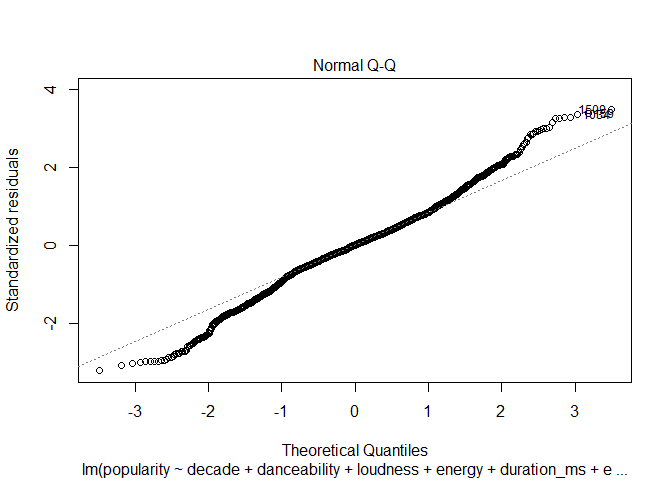 |
Plots of the residual versus the fitted values for the two proposed models.
Linearity From the above plot on the left of the residuals vs fitted values, we see no significant patterns or deviations from the middle, horizontal line, when the residuals have value of zero. Thus the residuals satisfy the linearity assumption.
Homoscedasticity The residuals are distributed fairly evenly above and below the zero line, and they have no distinct kinks or turns, including at the low and high ends of the fitted values. However, we see the residuals forming a straight, diagonal line at the fitted values of around 15 to 30, and the residual values of around -20 to -40. This may be due to the fact that the dependent variable, popularity, is from 0 to 100, and hence for a fitted value of, say, 20, it is impossible to have a residual smaller than -20. Aside from this quite minor problem, the residuals show a good degree of homoscedasticity.
Normality The above Q-Q plot shows a good degree of normality, aside from the tails of the plot, which see small kinks at either end, suggesting slightly heavier tails than a normal distribution. However, as these kinks are only small, we can still accept from this plot that the normality assumption is met.
Independence The independence assumption is checked by assessing the residuals, and seeing if any patterns with variables arise.
From the below plot, we see a clear pattern forming in the residuals. There seems to be a distinct hierarchy among the residuals, in that the residuals have formed “layers”, with The Beatles and Elvis having the highest popularity for a given value of one of our residuals, followed by Beyonce, David Bowie, Blur and Elvis, in that order. In general, these distinct layers seem to not be violated, which suggest that the residuals are not truly random. This makes sense, since if an artist has a popular song, this may affect the popularity of other songs on that album, meaning the samples aren’t truly independent, and hence the independence assumption is not satisfied.
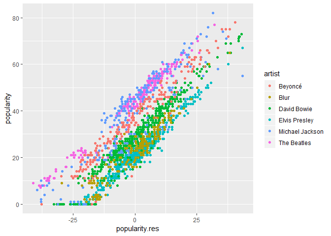
Scatter plot of model residuals vs popularity, by artist.
9 Prediction
Using the final model, the predicted popularity for a three minute song form the 90s in the key of C, with all other variables set to their sample mean, is 23.8. The confidence interval for this samples popularity is (21.25, 26.35)
10 Conclusion
Nine potential predictor variables were considered to enable the construction of a linear regression model that would enable the prediction of a song’s popularity. The data was loaded into the R Studio environment and examined for inconsistency. The dataset was adjusted to ensure a consistent and uniform database. Bi-variate and uni-variate analyses offered valuable insight into the type of data in the data set and relationships within the data set. Only two variables, Loudness and Energy, appeared strongly correlated.
Analysis of Variance was used to evaluate the significance of the relationship between variables and their second order interactions. Three different scopes were used when building models; one without any interaction terms, one with only the significant terms and one with all terms.Three different algorithms from model fitting were used; backward, forward and step-wise were applied in each of the previously outlined scopes. This was further expanded by using both the Akaike and Bayesian Information Criterion as heuristics. This resulted in 18 potential methods of obtaining fitted linear model. From this pool of models the general formula:
popularity ~ decade + danceability + loudness + energy + duration_ms + , energy:duration_ms + decade:loudness
was selected based on cross validated MSE score and model complexity. The assumptions for this model of linearity, homoscedasticity, normality and independence were checked with diagnostic plots. Although some of the assumption are support by these plots some underlying sampling bias prevents this model complying with the assumption of independence. In this way the model is likely to generalise poorly to other Artists than those not considered in this study. The model was then used to predict the popularity of a three minute song from the 90s in the Key of C, all other predictors are set to their respective mean or mode. Predicting a value of 23.80 with a 95% confidence interval of (21.25, 26.35). This model can be used to predict the popularity of any song given data ‘decade’, ‘danceability’, ‘loudness’, ‘energy’ and ‘duration’. Cross validating on the given data set, the final model scored 166.8 MSE (mean squared error), or 12.9 RMSE (root mean squared error), from the true popularity.
To expand upon the work done thus far random sampling of more songs would enable stronger assumptions about independence of residuals and promote diversity in training data and thus generalisation of the model. In addition to this more complex forms of modeling and analysis could be used to contrast the relatively simple model proposed. Although in general models that involve boosting or bagging will decrease the interpret-ability of the model.
References
RIAA. 2018. “U.S. Sales Database.” Recording Industry Association of America. https://www.riaa.com/u-s-sales-database/.
SpotifyAB. 2018. “Get Audio Features for a Track - Audio Features Object.” https://developer.spotify.com/documentation/web-api/reference/tracks/get-audio-features/.
[1] Recording Industry Association of America. U.S. Sales Database [Webpage]. Retrieved from https://www.riaa.com/u-s-sales-database/. Reported figures have been adjusted for inflation.
[2] SpotifyAB, Get Audio Features for a Track - Audio Features Object [Webpage]. Retrieved from https://developer.spotify.com/documentation/web-api/reference/tracks/get-audio-features/