Introduction
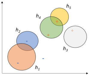
Ensemble learning methods take the perspective that by constructing a classifier that uses several hypothesises pooled together, it would be less likely to misclassify samples than any of the singular hypothesis acting on their own. Boosting is a specific case where the classifiers used in the ensemble are weighted and each subsequent classifier is trained on a modified dataset that penalises the previous classifiers correctly classified samples and rewards classification of the mistakes. Therefore, the final ensemble becomes a group of experts in particular areas of the space being classified. This creates a model which is able to compensate for other classifiers yielding a complete model. In the accompanying figure the coloured regions represent areas where a given hypothesis yields incorrect classifications. As an ensemble no three hypothesises are never wrong about a single point's classification, consequently three out of five classifiers are always correct. Therefore a majority vote from the collection of hypothesises will classify the samples in the space with 100% accuracy. There are many examples of algorithms that are based on the idea of boosting, in this document the processes and procedures used to adjust the weights of the samples in the dataset and form the ensemble are consistent with Adaptive Boosting also referred to as AdaBoost. This particular algorithm assumes that the ensemble of classifiers are examples of weak learners, which are only slightly better at classifying samples than randomly assigning them a label. When this assumption is met AdaBoost returns models that are guaranteed to classify the training set perfectly given a large enough ensemble size. It is also extremely resilient to over-fitting as a result of model complexity. In many cases it has been shown that accuracy on the testing set continues to increase as more hypothesis are added to the ensemble after the training classification has reached 100%. This seems to contradict the traditional rule of Ockham's razor utilised so frequently in modelling, where model complexity is penalised in order to ensure generalisation. [4] Here in, binary classification problems are considered, but the techniques can be extended to multi-class and regression problems. [2] To examine the AdaBoost algorithm first the mathematics behind the formation of the ensemble will be explored, then a prototype of the boosting algorithm will be implemented in Python and compared to an open source implementation. These results will then be compared to a Support Vector Machine to contrast the two classifiers respective strengths and weaknesses.
Adaptive Boosting
Initialisation
Weak Learners
As stated above, the weighted ensemble of learners that form the final classifier must fall into the category of weak learners. This gives any individual hypothesis an accuracy of \(0.5+\delta\), where \(\delta\) is the advantage the classifier has over random label assignment. The condition of weak learner is met by a large number of classifier type, but in this case the ensembles will be formed of decision stumps, due to their simplicity. Each stump is a classification rule with a threshold value and a respective dimension, where either +1 or -1 will be assigned to values above or below the threshold. Each stump will have a mirror stump in which the assignment of labels relative to the threshold is reversed.
# Decision stump classifier, if rightPos is true everything to the
# left of the threshold is assigned -1, to the right +1
# if rightPos is false label assignment is flipped
class Stump:

    def __init__(self, dimension, value, rightPos):
        self.dimension = dimension
        self.value = value
        self.rightPos = rightPos

    error = 1
    alpha = 0
Initialising a collection of possible decision stumps for the input data is the first step of the Adaptive Boosting algorithm as the learners that ultimately form the classifier will be drawn from this pool. In this case every possible unique split was considered when forming the hypothesis space. Each dimension is ordered, then duplicate values removed and two decision stumps are initialised at each of the midpoints between consecutive unique values in the dimension; one that labels the samples to the right as positive and another to labels to the left as positive. Additionally an extra two stumps are created that label all samples as positive or negative are initialised to. This leads to a large space of possible learners, \(2\sum_{i}^{d}n_{i}\) where \(n\) is the number of unique values in the \(i\)th dimension and \(d\) is the dimensionality of the feature space.\
# Takes in the dataframe and geenrates possible
# decision stumps for each dimension of the set
def generateStumps(dataFrame):
    # For each dimension (variable) order the data along it
    # find the midpoints between consecutive points
    # create a stump for each midpoint value

    tmpDF = dataFrame # Creates a copy of the data

    # Extract information about the data frame
    columns = list(tmpDF)
    numberOfVariables = dataFrame.shape[1]
    numberOfSamples = dataFrame.shape[0]

    # Multidemisionaly array of stumps
    allStumps = list()
    oneDStumps = list()

    # for each variable sort by it and make stumps
    # between points
    for i in range(1, numberOfVariables):
        # Sorts the samples in ascending order in the
        # desired dimension
        tmpDF.sort_values(by = [columns[i]])

        # Find the mid-point between sequentialy ordered samples
        # disregarding duplicate entries along the demision
        tmp = tmpDF.loc[0, columns[i]]

        for j in range(1, numberOfSamples):
            # Get the next largest value in the ith dimension
            tmpNext = tmpDF.loc[j, columns[i]]
            # Compare it to the previous
            if (tmp != tmpNext):
                newSplit = (tmpNext+tmp)/2
                newStump = Stump(i, newSplit, True)
                oneDStumps.append(newStump)
                newStump = Stump(i, newSplit, False)
                oneDStumps.append(newStump)
            # Get the next value in the dimension
            tmp = tmpNext

        # Add the generated stumps to the overall
        allStumps.append(oneDStumps)
        # Clear the oneDStump list
        oneDStumps = list()

    return allStumps
Sample Weights
Initially the samples weights need to form a uniform distribution, as the weights are a distribution they are subject to the law of total probability and are therefore constrained by: \[ \sum_{1=1}^{n} w_{i_{t}} = 1 \] Where \(n\) is the total number of samples in the set and t is the current iteration. As the distribution begins uniform all samples have the same weight, \(w_{i} = c\) for \(i = 0, 1, ... , n\) giving the initial value for each sample's weight as: \[ w_{i_{1}} = \frac{1}{n} \]
# Create an array of wieghts the same size as the data frame
# where each wieght starts at 1/n where n is the total number
# of samples
def initialiseWeights(dataFrame):
    numberOfVariables = dataFrame.shape[1] - 1
    numberOfSamples = dataFrame.shape[0]
    wieghts = np.ones((numberOfSamples))*(1/numberOfSamples)

    return wieghts
Iteration
Learner Selection - Error Evaluation
Each of the possible learners is evaluated against the weighted error of itself. To calculate the weighted error all the samples that are misclassified have their respective weights summed together: \[ \epsilon = \sum_{i=1}^{n} w_{i_{t}} \text{ for } h(x_{i}) \neq y(x_{i}) \] Where \(x_{i}\) is the sample, \(h(x_{i})\) is the classifiers label of the \(i\)th sample and \(y(x_{i})\) is the true label of the \(i\)th sample. The classifier for which this weighted error is minimised is selected from the space of possible learners. This classifier is then used in the final.
# Takes a sample and returns a label
def classify(self, sample):
    if self.rightPos:
        if (sample >= self.value):
            return +1
        else:
            return -1
    else:
        if (sample < self.value):
            return +1
        else:
            return -1

# Vectorisable method for evaluating errors,
# returns weight or zero
def vecError(self, sampleValue, label, weight):
	# Is the sample classified correctly
	if (classify(sample) == label):
    	return 0.0
    else:
    	return weight

# Vectorised evaluation of error
def evaluateError(self, dataFrame, sampleLabels, sampleWeights):
    # vectorise the error function
    vectorError = np.vectorize(self.vecError)
    errors = vectorError(dataFrame[:, self.dimension], sampleLabels, sampleWeights)
    # Sum up the array of wieghts for incorrectly classified samples
    self.error = np.sum(errors)
# For each of the possible decisions update their error
# then return the stump with the least error
def selectBestStump(possibleStumps, dataFrame, weights, labels):
    # Set the best stump to false
    bestStump = Stump('Null', 'Null', False)

    # Testing counter to see how many equivelent decisions exist
    counter = 0

    # Update the error of each possible stump
    for i in range(len(possibleStumps)):

        for j in range(len(possibleStumps[i])):
            possibleStumps[i][j].evaluateError(dataFrame.values, labels.values, weights)
            # If the current stump has lees error than the current best
            # update the current stump as the current best
            if (bestStump.value == 'Null'):
                bestStump = possibleStumps[i][j]
            else:
                if (possibleStumps[i][j].error < bestStump.error):
                    bestStump = possibleStumps[i][j]
                elif (possibleStumps[i][j].error == bestStump.error):
                    counter += 1

    return bestStump, counter
Weight of Classifier in Final Model
Once the best hypothesis has been select from the pool of possible, the weight of this classifier in the final model can be evaluated. This weight assignment is at the core of AdaBoost and is derived in order to ensure the overall error of the model is bounded by exponential loss. [1] The weight given to the \(i\)th classifier in the final model, \(\alpha_{i}\), is calculated by: \[ \alpha_{i} = \frac{1}{2}\ln{\left(\frac{1-\epsilon_{i}}{\epsilon_{i}}\right)} \]
# Updates the stump's alpha value
def updateAlpha(self):
    newAlpha = (1-self.error)/(self.error)
    newAlpha = np.log(newAlpha)
    newAlpha /= 2
    # Raptors got a new alpha
    self.alpha = newAlpha
Updated Sample Weights
Using the calculated classifier weight \({\alpha_{i}}\) the samples weight distribution is updated so on the next iteration the samples classified incorrectly by the current learner are rewarded more than those already classified correctly. To do this each weight is scaled by \(\alpha\), up for incorrectly classified samples and down for correctly classified: \[ w_{i_{t+1}} = \frac{w_{i_{t}}}{Z} \text{ }\alpha_{i} \text{ If } h(x_{i}) \neq y(x_{i}) \] \[ w_{i_{t+1}} = \frac{w_{i_{t}}}{Z \alpha_{i}} \text{ If } h(x_{i}) = y(x_{i}) \] Where \(Z\) is a normalisation term given by: \[ Z = 2\sqrt{\epsilon_{i}(1-\epsilon_{i})} \] The process is then repeated from the error evaluation step until the desired number of classifiers are found. Therefore, the final model will be in form of a linear sum of classification functions multiplied by their respective \(\alpha\). [3]
# Update the samples weights for the next classifier
def updateWeights(stump, weights, dataFrame, labels):
    # Use the stump to classify the set
    predictions = stump.classifySet(dataFrame.values)

    # Calculates Z the normalisation constant
    Z = 2*np.sqrt(stump.error*(1-stump.error))

    # Check which where correct/incorrect and update the
    # corresponding wieght
    for i in range(len(predictions)):
        if (labels[i] == predictions[i]):
            weights[i] /= np.exp(stump.alpha)
            weights[i] /= Z
        else:
            weights[i] *= np.exp(stump.alpha)
            weights[i] /= Z

    return weights
Classification
To classify a new sample as +1 or -1 using the model, each classifier is used on the sample sequentially with each classifiers prediction being multiplied by its respective alpha. This weighted prediction is then added to a cumulative summation. Once all the learners in the ensemble have contributed to the summation, is reduced to a label by taking the sign: \[ H(x) = \text{Sign}\left(\alpha_{1} h_{1}(x) + \alpha_{2} h_{2}(x) + \dots + \alpha_{j} h_{j}(x)\right) \]
 # Using the trained model, predict the classes of the data
    def predict(self, dataFrame):
        # Reset summation
        predictions = np.zeros(dataFrame.shape[0])

        # Get the wieghted prediction from each classifier in the model
        for classifier in self.model:
            # Classify and weight all samples by a classifier
            tmp = (classifier.alpha) * (classifier.classifySet(dataFrame.values))

            # Sum into the prediction
            predictions += tmp

        return np.sign(predictions)
Implementation
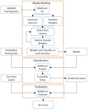
A prototype Adaptive Boosting algorithm was implemented in Python, using Jupyter notebook as the development environment. The prototype uses an implemented decision stump class to form the ensemble of learners. AdaBoost is then applied in order to train, select and weight classifiers, which construct the final model. To achieve this the work-flow in the figure to the right was used. Some aspects of the implementation were vectorised in order to reduce training time to a reasonable length. The major source of computation time comes from the nested loops which evaluate the error for each possible weak learner in the set of hypothesises.
# Accepts a pandas data frame and the number of iterations
# the algorithm of adaptive boosting before retuning the model
def train(self, dataFrame, labels, iterations):
    # Initialisation
    possibleStumps = generateStumps(dataFrame)
    weights = initialiseWeights(dataFrame)
    # Training the model
    for i in range(iterations):
        # Select the best classifier
        bestStump, counter = selectBestStump(possibleStumps, dataFrame, weights, labels)
        # Update its alpha value
        bestStump.updateAlpha()
        # Update the weights
        weights = updateWeights(bestStump, weights, dataFrame, labels)
        # Add best stump to the model
        self.model.append(bestStump)
Evaluation
To access the implemented algorithm two datasets were adapted from the UCI Machine Learning Repository. The first was reduced to a binary classification of emails as spam or not [8], the second are C and G samples from the letter image recognition database, [9]. On importing the datasets respective labels were encoded such that Cs are +1, Gs are -1 and Spam is -1, not spam is +1.
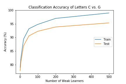
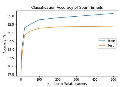
For both datasets the implemented algorithm achieved classification accuracies of over 90% when the ensemble consisted of 50 learners, see the below figures. The algorithm appears to be increasing towards a perfect model for the training data in both cases, but was yet to reach it with 500 learners in the model. Diminishing returns of accuracy form adding model complexity is evidenced clearly here, with the majority of testing accuracy increase seen in the first 50 learners, from this point increasing the ensemble size by ten fold the accuracy is observed to increase by 4% on the Letters data and 2% on Emails. It is important to note that with an increase of learners comes a corresponding increase in compute time as seen in the appended tables of results
 |  |
Throughout the implementation time complexity was identified as a significant factor in the ability to increase model complexity and is exacerbated by higher dimensionality and larger datasets. However there is a large amount of optimisation still available, as most of the operations are completed by generic loops and can be vectorised to leverage parallel processing. The room to develop is evidenced by the runtime results seen for the imported AdaBoost algorithm, evidenced in the appended tables. Towards this goal the space of possible hypothesises was considered as something that could be reduced. Currently the implemented algorithm conducts an exhaustive comparison based search on the set of all possible mid-points between sequential samples and their inverse labelling rules. Over the course of implementation emphasis was placed on the best possible decision stump being returned, but the error metric used to evaluate this is not guaranteed to be unique. The number of these redundancies changes as the algorithm progresses, but the maximum observed was 686 equivalent decisions when applied to the Letters dataset. Initially this was viewed as problematic and measures to separate which of the equivalent decisions are better were considered, but under the conditions of Adaptive Boosting it becomes clear that sub-optimal choices in learner have little overall impact on the accuracy of the model. This is likely a consequence of the assumption that the ensemble's learners should be weak in nature. Continuing this line of reasoning, informed reductions in the space of possible classifiers could be made without the loss of the ensembles classification power, or perhaps an early end to the search when the first decision that is suitably strong is found. Ultimately this will require further testing to investigate and will likely effect the rate of convergence on a perfect training model, perhaps trading search time for larger ensembles.\ The imported AdaBoost algorithm finds a model to fit the training data somewhere between 50-100 learners, seen in the below plots. It also shows a steeper ascent to this in comparison to the prototype. A feature of the imported algorithm is once a model that classifies the training data completely it will not add further learners to the ensemble. This is why the testing accuracy is shown to stagnate after the first model that gets 100% accuracy on the training data is found. The faster convergence of the model on a perfect fit is likely due to the variant of Adaptive Boosting the imported package uses Stage-wise Additive Modelling using a Multi-class Exponential loss function - Real (SAMME.R). [5] Although literature suggests this approach reduces to AdaBoost when the classification problem is binary, [7] the example in the packages documentation shows that on a binary classification problem SAMME and SAMME.R preform differently. [6]
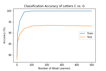 | 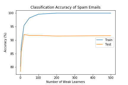 |
As the two datasets examined are seemingly non-linear in nature and contain high amounts of overlap the results of AdaBoost were compared with a Support Vector Machine (SVM). In this comparison the resistance that AdaBoost has to over fitting is clear. The imported SVM under hard-margin could not find a decision boundary for the linear or second degree polynomial kernel. A Gaussian kernel enables the formation of the decision boundary, but even when carefully tuned over-fits the dense overlapping feature space of the examined datasets, shown in the plots below. This achieved a maximum testing accuracy of 50% on the Letters dataset and 60% on the Emails. Even the efforts to maximise generalisation taken during the conception of SVMs over-fit on these dataset before reaching a decision rule that can perfectly classify the training set. Whereas AdaBoost's achieves exceptional classification accuracy and in these two examples, appearing experimentally immune to the negatives usually associated with increased model complexity.
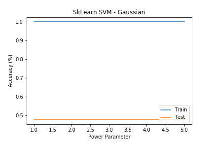 | 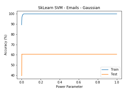 |
Adaptive Boosting - Tabulated Results
| Ensemble Size | Training Accuracy (%) | Testing Accuracy (%) | Training Time (s) | Testing Time (s) |
|---|---|---|---|---|
| 1 | 79.0 | 77.80 | 4.61 | 0.00 |
| 5 | 82.4 | 81.07 | 22.76 | 0.00 |
| 20 | 89.4 | 86.92 | 89.61 | 0.02 |
| 50 | 93.2 | 90.58 | 223.27 | 0.04 |
| 100 | 94.8 | 92.27 | 446.56 | 0.10 |
| 200 | 97.0 | 93.86 | 888.80 | 0.20 |
| 500 | 99.0 | 95.34 | 2228.55 | 0.47 |
Results of testing conducted using the implemented AdaBoost algorithm on the Letter recognition dataset.
| Ensemble Size | Training Accuracy (%) | Testing Accuracy (%) | Training Time (s) | Testing Time (s) |
|---|---|---|---|---|
| 1 | 80.6 | 77.92 | 22.75 | 0.00 |
| 5 | 84.6 | 82.34 | 111.37 | 0.01 |
| 20 | 91.5 | 89.28 | 446.63 | 0.05 |
| 50 | 92.5 | 90.50 | 1123.43 | 0.15 |
| 100 | 93.9 | 91.36 | 2247.44 | 0.34 |
| 200 | 94.5 | 91.78 | 4520.25 | 0.72 |
| 500 | 95.8 | 92.00 | 11259.84 | 1.71 |
Results of testing conducted using the implemented AdaBoost algorithm on the Emails dataset.
| Ensemble Size | Training Accuracy (%) | Testing Accuracy (%) | Training Time (s) | Testing Time (s) |
|---|---|---|---|---|
| 1 | 79.0 | 77.80 | 0.00 | 0.00 |
| 5 | 89.8 | 86.03 | 0.01 | 0.00 |
| 20 | 95.6 | 89.49 | 0.03 | 0.01 |
| 50 | 99.6 | 91.97 | 0.07 | 0.01 |
| 100 | 100.0 | 93.16 | 0.14 | 0.02 |
| 200 | 100.0 | 93.46 | 0.28 | 0.05 |
| 500 | 100.0 | 93.16 | 0.73 | 0.12 |
Results of testing conducted using sklearn’s AdaBoost algorithm on the Letter recognition dataset.
| Ensemble Size | Training Accuracy (%) | Testing Accuracy (%) | Training Time (s) | Testing Time (s) |
|---|---|---|---|---|
| 1 | 79.0 | 77.80 | 0.00 | 0.00 |
| 5 | 89.8 | 86.03 | 0.01 | 0.00 |
| 20 | 95.6 | 89.49 | 0.03 | 0.01 |
| 50 | 99.6 | 91.97 | 0.07 | 0.01 |
| 100 | 100.0 | 93.16 | 0.14 | 0.02 |
| 200 | 100.0 | 93.46 | 0.28 | 0.05 |
| 500 | 100.0 | 93.16 | 0.73 | 0.12 |
Results of testing conducted using sklearn’s AdaBoost algorithm on the Emails dataset.
References
[1] Breiman, L. 1997. “Predictions Games and Arcing Algorithms.” Technical Report 504, Statistics Department, University of California, December, 9–11.
[2] Freund, Y., and R. Schapire. 1997. “A Decision-Theoretic Generalization of on-Line Learning and an Application to Boosting.” Journal of Computer and System Sciences 55 (SS971504): 119–39.
[3] “A Short Introduction to Boosting.” Journal of Japanese Society for Artifical Intelligence 14 (5): 771–80, 1999
[4] Russell, S., and P. Norvig. 2010. Artificial Intelligence: A Modern Approach. Third. Pearson.
[5] Scikit-Learn. 2018a. “1.11.3 Adaboost.” Scikit-Learn. 2018. http://scikit-learn.org/stable/modules/ensemble.html#adaboost
[6] 2018b. “Discrete Versus Real Adaboost.” Scikit-Learn. 2018. http://scikit-learn.org/stable/auto_examples/ensemble/plot_adaboost_hastie_10_2.html
[7] Zhu, J., and H. Zou. 2009. “Multi-Class Adaboost.” Statistics and Its Interface 2: 349–60.
[8] M. Hopkins and E. Reeber, Spambase Data Set, University of California, Irvine, 1999 https://archive.ics.uci.edu/ml/datasets/Spambase
[9] D. Slate, Letter Image Recognition Data, University of California, Irvine, 1991 https://archive.ics.uci.edu/ml/machine-learning-databases/letter-recognition/`